GHz momentum computing simulation #1

August 18, 2025

nb: attempting a daily posting cadence as weekly clearly doesn't work. adjust quality priors accordingly

Momentum computing is, as far as I can tell, a reversible computing paradigm which circumvents Landauer's limit by embedding the memory state transitions of some computing device in a physical system which equilibriates slower than the time it takes to do an individual bit-swap, so that the memory state transitions themselves can store information in their "instantaneous momenta" and subsequently perform bit-swaps with near-zero net work.¹

In particular, one can construct toy theoretical energy potentials which implement a $\Delta W = 0$ Fredkin gate.² Consider a particle $(x,p)$ in the 1D potential $V_B(x) = \alpha x^4 - \beta x^2.$ The two minimal states are located at $x = \pm \sqrt{\beta / 2\alpha},$ and as transitioning from the $x < 0$ regime to the $x >0$ regime is exponentially prohibitive in the value of $V(0),$ the system "stores" a bit $\{0,1\}$ depending on the sign of the particle's position.

Now imagine that $V_B$ encodes a thermal bath in which the particle $(x,p)$ is embedded in, and assume that the particle's motion follows harmonic oscillation in the absence of external influence. When the bath is active, the particle's potential is described by $V_B.$ But when the bath is disengaged, the particle behaves according to $V_H(x) = kx^2/2,$ which induces a trajectory $x(t) = A \cos(t \sqrt{k/m} + \phi),$ which is periodic in time $\tau = 2\pi \sqrt{m/k}.$ Therefore, disengaging the bath for time $\tau/2$ swaps the sign of the particle's position, effectively performing a bit-swap.

This theoretical "bit-swap" comes at no work cost because there is no change in potential energy from time $0$ to $\tau/2.$³ However, any physical implementation of this concept must contend with the fact that changing the potentials in a physical system requires energy to be expended, likely in an inefficient manner. How does one get around this? Superconductors!

gradiometric flux logic cells

The theoretical guarantees above require complete & efficient decoupling of the system from the bath. You can get similar results by simply ensuring that the relevant computational timescale is significantly smaller than the energy flux rate between the system and its bath, so that "from the perspective of the computation" there is no coupling.

[RC22] chooses to implement such a system with gradiometric flux logic cells, a kind of circuit utilizing Josephson junctions designed particularly to withstand global magnetic noise fluctuations [I do not really understand GFLCs very well, that will be a topic for another day's post].

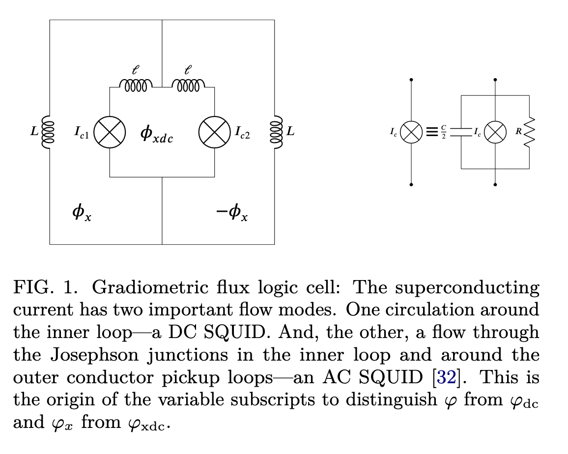
With suitable assumptions & parametrizations [such will be the subject of yet another day's post], the GFLCs follow "significantly underdamped Langevin dynamics", which can be described with the following equation: $$ dv' = -\lambda v'dt' - \theta \partial_{x'}U' + \nu r(t)\sqrt{2dt'} $$ where the potential $U$ evolves according to $$ U'(t') = (\phi-\phi_x(t'))^2/2 + \gamma(\phi_{dc} - \phi_{xdc}(t'))^2/2 + \beta \cos \phi \cos (\phi_{dc}/2) + \delta \beta \sin \phi \sin (\phi_{dc}/2) $$ where $x' = (\phi, \phi_{dc}), v' = (\dot{\phi}, \dot{\phi_{dc}})$, $\phi = (\phi_1 + \phi_2)/2 - \pi,$ $\phi_{dc} = (\phi_2 - \phi_1),$ and $\phi_1, \phi_2$ are the phases of the individual Josephson junctions $I_{c1}, I_{c2}$ in the above figure [I think]. $\phi_{x} = 2\pi \psi_x / \bf{\Phi}_0 - \pi$ and $\phi_{xdc} = 2\pi \psi_{xdc} / \bf{\Phi}_0$ are functions of the external magnetic fluxes $\psi_x, \psi_{xdc}$ applied to the circuit.

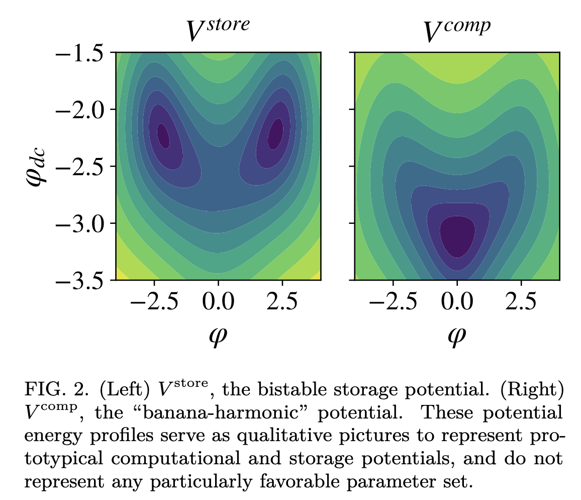
The details of this are very interesting, still confusing to me, and this is by no means an exhaustive parametrization of the underlying models. However, below (Fig. 2) showcases that varying $\phi$ and $\phi_{dc}$, the sum and difference of the Josephson phase parameters, recovers the potential geometry associated with costless bitswaps.

further considerations

• I really want to understand the interface between the theoretical dynamics and the physical implementation better. Why is this theory so substrate independent? Why does it matter that our memory state transitions are modeled by CTHMCs instead of CTMCs? Why are we using superconductors?
• How do we actually get efficient circuit modeling of the kind described here? I couldn't readily find a Github repository associated with the paper, so I want to write my own library and replicate their results. They find that the efficiency of their circuits are largely dependent on "circuit hyperparameters", and it would be interesting to investigate their structure.
• Benchmarks for algorithms that can be implemented with momentum computing and with typical CMOS/transistor logic, and developing simulations that can accurately predict efficiency differences. Still not sure how to think about this! Will absolutely be the topic of a later post.
• Fermi estimates of all the physical quantities at play here. What is "one Landauer" at STP? How much does it cost to make a gradiometric flux logic cell? Etc. Etc.

All credit goes to the coauthors of the two papers cited in this post.